Linear Regression
Least squares and gradient descent worked out by hand, with the partial derivatives written out and the model built up in code.
Overview
Linear regression is a method used in machine learning for predicting a continuous output variable based on one (univariate, or simple regression) or more (multiple linear regression) input features . The linear regression model is defined as:
where is the input feature vector, is the vector/scalar of model parameters (weights and the bias, and f is the predicted output value.
- is a vector in case of multiple linear regression. If there’s a single feature (univariate), the is a scalar.
- is always a scalar.
Mean Squared Error
To train the linear regression model, we need to minimize a cost function that measures the difference between the predicted output values and the true output values. The cost function for linear regression is the mean squared error, which is defined as:
where is the number of training examples, is the vector of true output values, and is the predicted output value defined above.
Calculating Partial Derivatives
To minimize the cost function, we need to find the values of that minimize the cost. We do this by taking partial derivatives of the cost function with respect to the parameters:
Partial derivative of cost function J w.r.t. the weights:
Partial derivative of cost function J w.r.t. the bias:
Gradient Descent
We can update the values of iteratively using gradient descent, which is a method that takes steps in the direction of the negative gradient of the cost function. The update equation for each parameter is:
where is the learning rate, which controls the size of the steps we take in each iteration.
This translates to:
where, parameters , are updated simultaneously.
Here simultaniously means that you calculate the partial derivatives for all the parameters before updating any of the parameters.
Improving the model
Feature scaling
Feature scaling is a preprocessing step that can be applied to the features (input variables) in a regression problem to ensure that they are on a similar scale.
When the features are on very different scales, algorithm may have difficulty converging to the optimal solution, and it may take longer to train the model. In addition, features with larger values may dominate the optimization process and have a disproportionate impact on the model’s predictions.
There are two common methods for feature scaling:
Standardization (Z-score): This method scales the features so that they have zero mean and unit variance. The formula for standardization is:
where is the original feature vector, is the standardized feature vector, is the mean of , and is the standard deviation of .
Normalization: This method scales the features so that they have a range between 0 and 1. The formula for normalization is:
where is the original feature vector, is the normalized feature vector, is the minimum value of , and is the maximum value of .
Both standardization and normalization can be effective in improving the performance of linear regression models by ensuring that the features are on a similar scale and have a similar impact on the model’s predictions. The choice of scaling method may depend on the specific problem and the characteristics of the data.
Feature engineering
Feature engineering is the process of creating new features from existing data that may improve the performance of a machine learning model. It involves selecting, transforming, and combining input features to create new features that are more informative or easier for the model to learn from.
Here are some common techniques for feature engineering in the context of linear regression:
Feature selection: This involves selecting a subset of the available features that are most relevant to the target variable. This can be done manually based on domain knowledge, or using automated methods such as regularization or feature importance measures.
Polynomial features: This involves creating new features by combining existing features using polynomial functions. For example, if there are two input features x and y, we can create a new feature by multiplying them together. We can also create higher-order polynomial features such as or .
Interaction terms: This involves creating new features by multiplying pairs of existing features. For example, if there are two input features and , we can create a new feature by multiplying them together. This can capture complex relationships between features that may be important for the target variable.
Encoding categorical variables: If the input features include categorical variables, they need to be encoded in a way that the linear regression model can understand. This can be done using one-hot encoding or other encoding techniques that convert the categorical variable into numerical features.
Scaling: Feature scaling can be used to ensure that the input features are on a similar scale. This can be important for linear regression models that use regularization or other methods that depend on the magnitude of the input features.
By carefully selecting, transforming, and combining input features, feature engineering can help improve the performance of linear regression models and enable them to better capture the underlying patterns in the data.
Choosing the correct learning rate ()
Choosing the correct learning rate is a crucial step in training machine learning models, including those based on gradient descent. A learning rate that is too low can result in slow convergence, while a learning rate that is too high can result in oscillations or even divergence. Here are some strategies for choosing a suitable learning rate:
Grid search: One approach is to use a grid search to try a range of learning rates and select the one that gives the best performance on a validation set. This can be time-consuming, but it is a straightforward way to find a good learning rate.
Learning rate schedules: Another approach is to use a learning rate schedule that adjusts the learning rate during training. For example, a common approach is to start with a high learning rate and gradually decrease it as the training progresses. This can help the model converge faster and avoid overshooting the optimal solution.
Adaptive learning rates: Some optimization algorithms, such as AdaGrad, Adam, and RMSprop, use adaptive learning rates that automatically adjust the learning rate based on the gradients observed during training. These algorithms can be more robust to different learning rates and may require less tuning.
Visualization: A simple way to diagnose the learning rate is to plot the training loss against the number of iterations or epochs for different learning rates. A good learning rate should result in a smooth decrease in the loss over time, without oscillations or instability. If the loss is not decreasing or is oscillating, the learning rate may be too high, and if the decrease is too slow, the learning rate may be too low.
In general, choosing the right learning rate can be a trial-and-error process that depends on the specific model, dataset, and optimization algorithm. It is important to monitor the training progress and adjust the learning rate as needed to ensure that the model is converging to a good solution.
Examples
# import data

import numpy as np
import matplotlib.pyplot as plt
import sklearn.datasets as dt
from sklearn import linear_model, model_selection
Univariate Linear Regression
This example shows the data generation, model building and prediction based on a single feature (input). It produces a straight line that best fits the data.
# generate random data
n_features = 1
n_samples = 1000
X, y = dt.make_regression(n_samples=n_samples, n_features=n_features, noise=10, random_state=1)

# split to train/test
X_train, X_test, y_train, y_test = model_selection.train_test_split(X, y, test_size=0.2)
print(X_train.shape, X_test.shape, y_train.shape, y_test.shape)
(800, 1) (200, 1) (800,) (200,)# create a model
sgdr = linear_model.SGDRegressor()# fit the model
sgdr.fit(X_train, y_train)
# print values of w and b and score
score = sgdr.score(X_train,y_train)
w = sgdr.coef_
b = sgdr.intercept_
print(f'Score = {score}\nWeights = {w}\nBias = {b}')Score = 0.9309201768687821
Weights = [38.35743486]
Bias = [0.3246334]# predict test data
pred = sgdr.predict(X_test)# visualize
plt.plot(X_test, pred)
plt.xlabel('input X')
plt.ylabel('f_w,b(x)')
plt.scatter(X_test, y_test, color='red')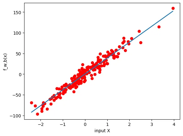
Multiple Linear Regression
This example shows how to use linear regression with multiple features. you can control the number of features in the dataset by changing the value of n_features below. The default number of features is 2, so we can visualize that on the chart. Each extra feature adds a dimension to the vizualization, so a single feature will consist of x y (2D graph - the plot will render a single line), and 2 features will be x1 x2 and y (3D graph - the plot will render a plane). As humans, 3D is the highest number of dimensions we’re comfortable with when viewing, so that’s what I went for.
# generate random data
n_samples = 10000
n_features = 2
X, y = dt.make_regression(n_samples=n_samples, n_features=n_features, noise=10, random_state=1)

# split into train/test
X_train, X_test, y_train, y_test = model_selection.train_test_split(X, y, test_size=0.2)
print(X.shape)
print(X_train.shape, y_train.shape, X_test.shape, y_test.shape)
(10000, 2)
(8000, 2) (8000,) (2000, 2) (2000,)# transform the test data
x_ = X[:,0]
y_ = X[:,1]
z_ = y
number_of_elements=100
# this will return evenly spaced numbers between x min and x max values
x_linspace = np.linspace(x_.min(), x_.max(), number_of_elements)
y_linspace = np.linspace(y_.min(), y_.max(), number_of_elements)
x_mesh, y_mesh = np.meshgrid(x_linspace, y_linspace)
model_viz = np.array([x_mesh.flatten(), y_mesh.flatten()]).T
print(X.shape, y.shape)
print(x_linspace.shape)
print(y_linspace.shape)
print(x_mesh.shape)
print(y_mesh.shape)
print(model_viz.shape)(10000, 2) (10000,)
(100,)
(100,)
(100, 100)
(100, 100)
(10000, 2)# create a model
sgdr = linear_model.SGDRegressor()
# fit the model
sgdr.fit(X, y)
# print the score
w = sgdr.coef_
b = sgdr.intercept_
score = sgdr.score(X, y)
print(f'Score = {score}\nWeights = {w}\nBias = {b}')Score = 0.9706498758188014
Weights = [30.64209408 48.37725872]
Bias = [-0.13509588]# predict for X_test
pred = sgdr.predict(model_viz)
# print predictions
print(pred[:2])
print(model_viz[:2])
print(np.dot(model_viz[:2], w) + b)[-282.78185712 -280.46721772]
[[-3.45140291 -3.6564401 ]
[-3.37586501 -3.6564401 ]]
[-282.78185712 -280.46721772]# visualize
plt.style.use('default')
fig = plt.figure(figsize=(12, 4))
ax1 = fig.add_subplot(131, projection='3d')
ax2 = fig.add_subplot(132, projection='3d')
ax3 = fig.add_subplot(133, projection='3d')
axes = [ax1, ax2, ax3]
for ax in axes:
ax.plot(x_, y_, z_, color='red', zorder=15, linestyle='none', marker='o', alpha=0.5)
ax.scatter(x_mesh.flatten(), y_mesh.flatten(), pred, facecolor=(0, 0, 0, 0), s=20, edgecolor='#70b3f0')
ax.set_xlabel('x[0]', fontsize=12)
ax.set_ylabel('x[1]', fontsize=12)
ax.set_zlabel('y', fontsize=12)
ax.locator_params(nbins=4, axis='x')
ax.locator_params(nbins=5, axis='x')
ax1.text2D(0.2, 0.32, 'aegis4048.github.io', fontsize=13, ha='center', va='center',
transform=ax1.transAxes, color='grey', alpha=0.5)
ax2.text2D(0.3, 0.42, 'aegis4048.github.io', fontsize=13, ha='center', va='center',
transform=ax2.transAxes, color='grey', alpha=0.5)
ax3.text2D(0.85, 0.85, 'aegis4048.github.io', fontsize=13, ha='center', va='center',
transform=ax3.transAxes, color='grey', alpha=0.5)
ax1.view_init(elev=27, azim=112)
ax2.view_init(elev=16, azim=-51)
ax3.view_init(elev=60, azim=165)
fig.suptitle('$R^2 = %.2f$' % score, fontsize=20)
fig.tight_layout()
plt.show()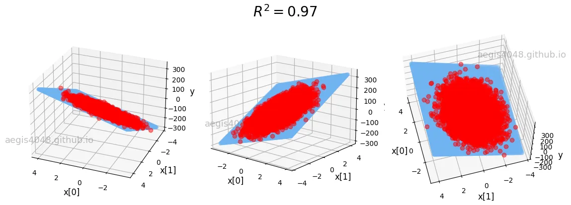
Plane sample
The below is just a way of presenting what values affect which parts of the plane when plotting. I had a little trouble understanding the above plots at first, so I decided to prep something like you see below.
fig = plt.figure(figsize=(16, 8))
ax = fig.add_subplot(131, projection='3d')
ax.set_xlabel('x[0]')
ax.set_ylabel('x[1]')
ax.set_zlabel('y_hat')

def plot(x, color):
  w_=0
  b_=0
  f_wb = np.dot(x, w_) + b_
  ax.plot(xs=x[0], ys=x[1], zs=f_wb[0], color=color, zorder=15, linestyle='none', marker='o', alpha=0.5)

plot([0, 0], 'red')
plot([0, 50], 'red')
plot([0, 100], 'red')
plot([50, 0], 'blue')
plot([50, 50], 'blue')
plot([50, 100], 'blue')
plot([100, 0], 'green')
plot([100, 50], 'green')
plot([100, 100], 'green')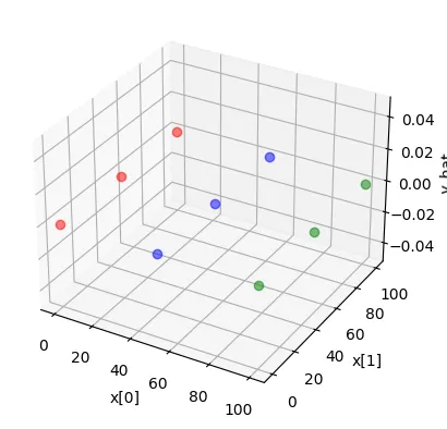
The below is the extension of the above example, but this time we’re using np.linspace and np.meshgrid to generate required data instead of hardcoding it.
import sys
np.set_printoptions(threshold=sys.maxsize)

fig = plt.figure(figsize=(16, 8))
ax = fig.add_subplot(131, projection='3d')
ax.set_xlabel('x[0]')
ax.set_ylabel('x[1]')
ax.set_zlabel('y_hat')

num_of_elements=100
x0__ = np.linspace(0, 100, num_of_elements)
x1__ = np.linspace(0, 100, num_of_elements)
x_mesh, y_mesh = np.meshgrid(x0__, x1__)

mid_x = int(num_of_elements/2)
mid_y = int(len(y_mesh.flatten())/2)
plot([x_mesh.flatten()[0], y_mesh.flatten()[0]], color='red')
plot([x_mesh.flatten()[0], y_mesh.flatten()[mid_y]], color='red')
plot([x_mesh.flatten()[0], y_mesh.flatten()[-1]], color='red')

plot([x_mesh.flatten()[mid_x], y_mesh.flatten()[0]], color='green')
plot([x_mesh.flatten()[mid_x], y_mesh.flatten()[mid_y]], color='green')
plot([x_mesh.flatten()[mid_x], y_mesh.flatten()[-1]], color='green')

plot([x_mesh.flatten()[-1], y_mesh.flatten()[0]], color='yellow')
plot([x_mesh.flatten()[-1], y_mesh.flatten()[mid_y]], color='yellow')
plot([x_mesh.flatten()[-1], y_mesh.flatten()[-1]], color='yellow')

plt.show()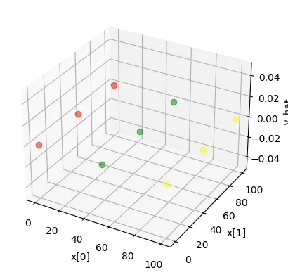
Linear Regression using PyTorch
import torch
import torch.nn as nn

class LinearRegressor(nn.Module):
  def __init__(self, in_dim, out_dim):
    super().__init__()
    self.lin = nn.Linear(in_dim, out_dim, device=device)

  def forward(self, x):
    return self.lin(x)

device = torch.device('cuda' if torch.cuda.is_available() else 'cpu')
print(device)

X_train = torch.tensor([[1],[2],[3],[4],[5]], dtype=torch.float32, device=device)
y = torch.tensor([[4],[7],[10],[13],[16]], dtype=torch.float32, device=device)
X_test = torch.tensor([10], dtype=torch.float32, device=device)

_, n_features = X_train.shape
_, n_targets = y.shape
model = LinearRegressor(n_features, n_targets).to(device)

print(f'prediction before the training - f({X_test.item()}) = {model(X_test).item():.3f}')

lr = 0.01
epochs = 1000
loss_fn = nn.MSELoss()
optimizer = torch.optim.SGD(model.parameters(), lr=lr)
for epoch in range(epochs):

  # forward pass - prediction
  y_pred = model(X_train)

  # calculate loss
  loss = loss_fn(y_pred, y)

  # backward pass - compute gradients
  loss.backward()

  # update weights
  optimizer.step()

  # reset gradients
  optimizer.zero_grad()

  if (epoch+1) % 100 == 0:
    w, b = model.parameters()
    print(f'epoch {epoch+1}: w = {w.item():.3f}, b = {b.item():.3f}, loss = {loss.item():.3f}')

print(f'prediction after training: f({X_test}) = {model(X_test).item():.3f}')
cpu
prediction before the training - f(10.0) = -6.523
epoch 100: w = 3.043, b = 0.845, loss = 0.004
epoch 200: w = 3.031, b = 0.889, loss = 0.002
epoch 300: w = 3.022, b = 0.921, loss = 0.001
epoch 400: w = 3.016, b = 0.944, loss = 0.001
epoch 500: w = 3.011, b = 0.960, loss = 0.000
epoch 600: w = 3.008, b = 0.971, loss = 0.000
epoch 700: w = 3.006, b = 0.980, loss = 0.000
epoch 800: w = 3.004, b = 0.985, loss = 0.000
epoch 900: w = 3.003, b = 0.990, loss = 0.000
epoch 1000: w = 3.002, b = 0.993, loss = 0.000
prediction after training: f(tensor([10.])) = 31.013