Logistic Regression
Sigmoid, log loss, regularisation and gradient descent for binary classification, worked through with code and plots.
Logistic regression is a machine learning algorithm used for binary classification problems, where the goal is to predict the probability of an event occurring (such as a customer buying a product or a patient being diagnosed with a disease) based on one or more input features.
Sigmoid function as
Logistic regression doesn’t output a single continuous variable like Linear Regression. Instead, the output is categorical, or binary. It outputs a 0 or a 1. We use sigmoid function to achieve that, which is defined as:
You can recall that the function is the function we normally use for linear regression. It’s a fundamental equation in machine learning - simply a function returning a straight line.
Loss
Unlike Linear Regression, using a Mean Squared Error won’t be a good choice for the loss function when we’re aiming at the non-linear function . Logistic Regression uses a loss function more suited to the task of categorization where the target is 0 or 1 rather than any number.
Loss is a measure of the difference of a single example to its target value while the
Cost is a measure of the losses over the training set
This is defined:
- is the cost for a single data point, which is:
-
is the model’s prediction, while is the target value.
-
where function is the sigmoid function.
The defining feature of this loss function is the fact that it uses two separate curves. One for the case when the target is zero or () and another for when the target is one (). Combined, these curves provide the behavior useful for a loss function, namely, being zero when the prediction matches the target and rapidly increasing in value as the prediction differs from the target. Consider the curves below:
The loss function above can be rewritten to be easier to implement.
This is a rather formidable-looking equation. It is less daunting when you consider can have only two values, 0 and 1. One can then consider the equation in two pieces:
when , the left-hand term is eliminated:
and when , the right-hand term is eliminated:
OK, with this new logistic loss function, a cost function can be produced that incorporates the loss from all the examples.
Cost Function
Recall, loss is defined to apply to one example. Here you combine the losses to form the cost, which includes all the examples.
Recall that for logistic regression, the cost function is of the form
where
- is the cost for a single data point, which is:
- where m is the number of training examples in the data set and:
Regularization
To prevent overfitting and improve the generalization performance of the model, we can add regularization terms to the cost function:
where is the regularization parameter that controls the strength of regularization, and is the number of features. Ridge (L2) and Lasso (L1) are two common types of regularization used in logistic regression.
Cost function for regularized logistic regression
For regularized logistic regression, the cost function is of the form
where:
Compare this to the cost function without regularization (which you implemented in a previous lab):
As was the case in linear regression above, the difference is the regularization term, which is
Including this term encourages gradient descent to minimize the size of the parameters. Note, in this example, the parameter is not regularized. This is standard practice.
Gradient descent with regularization
The basic algorithm for running gradient descent does not change with regularization, it is:
Where each iteration performs simultaneous updates on for all .
What changes with regularization is computing the gradients.
Computing the Gradient with regularization (both linear/logistic)
The gradient calculation for both linear and logistic regression are nearly identical, differing only in computation of .
-
m is the number of training examples in the data set
-
is the model’s prediction, while is the target
-
For a linear regression model
-
For a logistic regression model
where is the sigmoid function:
The term which adds regularization is the .
Evaluation Metrics
In binary classification problems, we typically use evaluation metrics such as accuracy, precision, recall, and F1 score to assess the performance of the model. These metrics can be calculated from the confusion matrix, which shows the number of true positive, true negative, false positive, and false negative predictions made by the model.
Here are some common evaluation metrics:
Accuracy: the proportion of correct predictions out of the total number of predictions.
Precision: the proportion of true positive predictions out of the total number of positive predictions. Recall: the proportion of true positive predictions out of the total number of actual positive instances.
F1 score: the harmonic mean of precision and recall, which gives equal weight to both metrics.
Conclusion
Logistic regression is a powerful and widely used algorithm for binary classification problems. By modeling the probability of the positive class as a function of the input features, logistic regression can make accurate predictions and provide insights into the underlying relationships between the variables.
Examples
Training a model on hand-written data
import numpy as np
import matplotlib.pyplot as plt
import matplotlib

X = np.array([[0.5, 1.5], [1,1], [1.5, 0.5], [3, 0.5], [2, 2], [1, 2.5]])
y = np.array([0, 0, 0, 1, 1, 1])

from sklearn.linear_model import LogisticRegression

lr_model = LogisticRegression()
lr_model.fit(X, y)

y_pred = lr_model.predict(X)

print("Prediction on training set:", y_pred)
print("Accuracy on training set:", lr_model.score(X, y))
Prediction on training set: [0 0 0 1 1 1]
Accuracy on training set: 1.0plt.scatter(X[:,0],X[:,1],c=y)
plt.scatter(X[:,0],X[:,1],c=y_pred)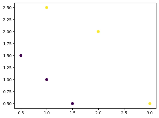
Generating synthetic data
Src: https://stackabuse.com/generating-synthetic-data-with-numpy-and-scikit-learn/
import sklearn.datasets as dt

fig,ax = plt.subplots(nrows=1, ncols=3,figsize=(16,5))
plt_ind_list = np.arange(3)+131
rand_state=1
color_map_discrete = matplotlib.colors.LinearSegmentedColormap.from_list("", ["red","cyan","magenta","blue"])

for class_sep,plt_ind in zip([0.1,1,10],plt_ind_list):
    x,y = dt.make_classification(n_samples=1000,
                                 n_features=2,
                                 n_repeated=0,
                                 class_sep=class_sep,
                                 n_redundant=0,
                                 random_state=rand_state)

    plt.subplot(plt_ind)
    my_scatter_plot = plt.scatter(x[:,0],
                                  x[:,1],
                                  c=y,
                                  vmin=min(y),
                                  vmax=max(y),
                                  s=35,
                                  cmap=color_map_discrete)
    plt.title('class_sep: '+str(class_sep))

fig.subplots_adjust(hspace=0.3,wspace=.3)
plt.suptitle('make_classification() With Different class_sep Values',fontsize=20)
plt.show()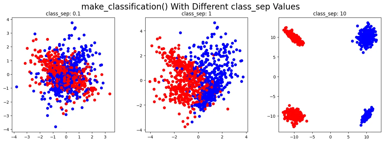
Training a model on synthetic data
from sklearn.model_selection import train_test_split

x,y = dt.make_classification(n_samples=10000,
                                 n_features=2,
                                 n_repeated=0,
                                 class_sep=3,
                                 n_redundant=0,
                                 random_state=rand_state)

plot = plt.scatter(x[:,0],
                    x[:,1],
                    c=y,
                    vmin=min(y),
                    vmax=max(y),
                    s=35,
                    cmap=color_map_discrete)
plt.title('classification data')
print(plot)
print(x.shape, y.shape)
x_train, x_, y_train, y_ = train_test_split(x, y, test_size=0.4)
x_cv, x_test, y_cv, y_test = train_test_split(x_, y_, test_size=0.5)
del x_, y_
print('x_train: ', x_train.shape, y_train.shape)
print('x_cv: ', x_cv.shape, y_cv.shape)
print('x_test: ', x_test.shape, y_test.shape)
model = LogisticRegression()
model.fit(x_train,y_train)
y_pred_train = lr_model.predict(x_train)
y_pred_cv = lr_model.predict(x_cv)
y_pred_test = lr_model.predict(x_test)

# print("Prediction on training set:", y_pred_train)
print("Accuracy on training set:", model.score(x_train, y_train))

# print("Prediction on CV set:", y_pred_cv)
print("Accuracy on CV set:", model.score(x_cv, y_cv))

# print("Prediction on test set:", y_pred_test)
print("Accuracy on test set:", model.score(x_test, y_test))
<matplotlib.collections.PathCollection object at 0x7f53796ef880>
(10000, 2) (10000,)
x_train: (6000, 2) (6000,)
x_cv: (2000, 2) (2000,)
x_test: (2000, 2) (2000,)
Accuracy on training set: 0.9945
Accuracy on CV set: 0.9955
Accuracy on test set: 0.9935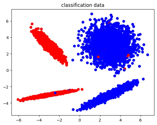
Plotting functions used by Logistic Regression
Sigmoid
# F_w,b(x) function plot

def sigmoid(x):
  return 1 / (1 + np.e ** -(x))

X = np.arange(-10, 10)
y = [sigmoid(x) for x in X]


plt.title('Sigmoid function')
plt.xlabel('X')
plt.ylabel('f(X) [sigmoid]')
plt.plot(X, y)
[<matplotlib.lines.Line2D at 0x7f5379488d30>]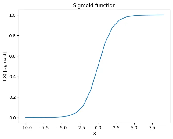
Log loss AKA Binary Cross-Entropy Loss:
from sklearn.metrics import log_loss

# target is 0
y_pred = np.linspace(0,1,1000) #np.array([0.1, 0.2, 0.3, 0.4, 0.5, 0.6, 0.7, .8, .9])
m = len(y_pred)
y = np.zeros(m)
losses = []
for i in range(m):
  loss = log_loss([y[i]], [y_pred[i]], labels=[0,1])
  losses.append(loss)


# target is 1
y_pred2 = y_pred.copy()
y2 = np.ones(m)
losses2 = []
for i in range(m):
  loss = log_loss([y2[i]], [y_pred2[i]], labels=[0,1])
  losses2.append(loss)  # loss = log_loss()
plt.title('Log loss')
plt.plot(y_pred, losses, color='red', label='0 target')
plt.plot(y_pred2, losses2, color='green', label='1 target')
plt.xlabel('y^ (predicted y)')
plt.ylabel('Log loss(y^)')
plt.legend(loc="upper left")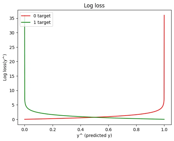
Logistic Regression using Neural Networks
import tensorflow as tf


X, y = dt.make_classification(n_samples=10000,n_features=5, n_classes=2, class_sep=10, n_repeated=0, n_redundant=0, random_state=7)
print(X.shape, y.shape)
print(X[0], y[0])
print(plt.scatter(X[:,0], X[:,1], c=y))

X_train, X_, y_train, y_ = train_test_split(X, y, test_size=0.4)
X_test, X_cv, y_test, y_cv = train_test_split(X_, y_, test_size=0.5)
print('train shapes: ', X_train.shape, y_train.shape)
print('CV shapes: ', X_cv.shape, y_cv.shape)
print('test shapes: ', X_test.shape, y_test.shape)


model = tf.keras.Sequential([
    tf.keras.layers.InputLayer(input_shape=(None,5)),
    tf.keras.layers.Dense(4, name='1'),
    tf.keras.layers.Activation('linear'),
    tf.keras.layers.Dense(4, name='2'),
    tf.keras.layers.Activation('linear'),
    tf.keras.layers.Dense(2, name='3'),
    tf.keras.layers.Activation('linear'),
    # tf.keras.layers.Dense(4, activation='linear', name='1'),
    # tf.keras.layers.Dense(4, activation='linear', name='2'),
    # tf.keras.layers.Dense(2, activation='linear', name='3')
])
model.compile(
    optimizer=tf.keras.optimizers.Adam(),
    loss=tf.keras.losses.BinaryCrossentropy()
)

model.fit(X_train, y_train, epochs=10)
print('-----')
model.evaluate(X_train, y_train)
print('-----')
model.evaluate(X_cv, y_cv)
print('-----')
model.evaluate(X_test, y_test)
(10000, 5) (10000,)
[-1.06543586e+01 -3.89862449e-01 -8.96784598e+00 -5.63230234e-01
4.18771860e-03] 0
<matplotlib.collections.PathCollection object at 0x7f538852eef0>
train shapes: (6000, 5) (6000,)
CV shapes: (2000, 5) (2000,)
test shapes: (2000, 5) (2000,)
Epoch 1/10
188/188 [==============================] - 1s 2ms/step - loss: 4.0456
Epoch 2/10
188/188 [==============================] - 0s 2ms/step - loss: 3.8270
Epoch 3/10
188/188 [==============================] - 0s 2ms/step - loss: 3.8267
Epoch 4/10
188/188 [==============================] - 0s 2ms/step - loss: 3.8266
Epoch 5/10
188/188 [==============================] - 0s 2ms/step - loss: 3.8266
Epoch 6/10
188/188 [==============================] - 0s 2ms/step - loss: 3.8266
Epoch 7/10
188/188 [==============================] - 0s 2ms/step - loss: 3.8266
Epoch 8/10
188/188 [==============================] - 0s 2ms/step - loss: 3.8266
Epoch 9/10
188/188 [==============================] - 0s 2ms/step - loss: 3.8266
Epoch 10/10
188/188 [==============================] - 0s 2ms/step - loss: 3.8266
-----
188/188 [==============================] - 1s 2ms/step - loss: 3.8266
-----
63/63 [==============================] - 0s 2ms/step - loss: 3.8301
-----
63/63 [==============================] - 0s 2ms/step - loss: 4.06814.068141937255859
model.summary()Model: "sequential_10"
_________________________________________________________________
Layer (type) Output Shape Param #
=================================================================
1 (Dense) (None, None, 4) 24
activation_12 (Activation) (None, None, 4) 0
2 (Dense) (None, None, 4) 20
activation_13 (Activation) (None, None, 4) 0
3 (Dense) (None, None, 2) 10
activation_14 (Activation) (None, None, 2) 0
=================================================================
Total params: 54
Trainable params: 54
Non-trainable params: 0
_________________________________________________________________model.get_config(){'name': 'sequential_10',
'layers': [{'class_name': 'InputLayer',
'config': {'batch_input_shape': (None, None, 5),
'dtype': 'float32',
'sparse': False,
'ragged': False,
'name': 'input_9'}},
{'class_name': 'Dense',
'config': {'name': '1',
'trainable': True,
'dtype': 'float32',
'units': 4,
'activation': 'linear',
'use_bias': True,
'kernel_initializer': {'class_name': 'GlorotUniform',
'config': {'seed': None}},
'bias_initializer': {'class_name': 'Zeros', 'config': {}},
'kernel_regularizer': None,
'bias_regularizer': None,
'activity_regularizer': None,
'kernel_constraint': None,
'bias_constraint': None}},
{'class_name': 'Activation',
'config': {'name': 'activation_12',
'trainable': True,
'dtype': 'float32',
'activation': 'linear'}},
{'class_name': 'Dense',
'config': {'name': '2',
'trainable': True,
'dtype': 'float32',
'units': 4,
'activation': 'linear',
'use_bias': True,
'kernel_initializer': {'class_name': 'GlorotUniform',
'config': {'seed': None}},
'bias_initializer': {'class_name': 'Zeros', 'config': {}},
'kernel_regularizer': None,
'bias_regularizer': None,
'activity_regularizer': None,
'kernel_constraint': None,
'bias_constraint': None}},
{'class_name': 'Activation',
'config': {'name': 'activation_13',
'trainable': True,
'dtype': 'float32',
'activation': 'linear'}},
{'class_name': 'Dense',
'config': {'name': '3',
'trainable': True,
'dtype': 'float32',
'units': 2,
'activation': 'linear',
'use_bias': True,
'kernel_initializer': {'class_name': 'GlorotUniform',
'config': {'seed': None}},
'bias_initializer': {'class_name': 'Zeros', 'config': {}},
'kernel_regularizer': None,
'bias_regularizer': None,
'activity_regularizer': None,
'kernel_constraint': None,
'bias_constraint': None}},
{'class_name': 'Activation',
'config': {'name': 'activation_14',
'trainable': True,
'dtype': 'float32',
'activation': 'linear'}}]}Single layer operations
d = model.get_layer('1')
weights, biases = d.get_weights()
print(weights.shape, biases.shape)
(5, 4) (4,)data = np.linspace(0, 1, num=5*4).reshape(4, 5)
dataarray([[0. , 0.05263158, 0.10526316, 0.15789474, 0.21052632],
[0.26315789, 0.31578947, 0.36842105, 0.42105263, 0.47368421],
[0.52631579, 0.57894737, 0.63157895, 0.68421053, 0.73684211],
[0.78947368, 0.84210526, 0.89473684, 0.94736842, 1. ]])d.call(tf.convert_to_tensor(data))<tf.Tensor: shape=(4, 4), dtype=float32, numpy=
array([[ 0.12562466, -0.06933554, -0.19231609, -0.22665459],
[ 0.35527048, -0.02021147, -0.4000274 , -0.5530683 ],
[ 0.58491623, 0.02891259, -0.6077387 , -0.879482 ],
[ 0.8145621 , 0.07803667, -0.81544995, -1.2058957 ]],
dtype=float32)>print(weights)
print('-------')
print(biases)[[ 0.0039245 0.5996987 0.47247538 0.02673925]
[ 0.20032103 0.10050099 0.13618797 0.1157181 ]
[ 0.276282 -0.23740293 -0.69783294 -0.65762925]
[ 0.01720777 -0.09424362 -0.4920638 -0.08301245]
[ 0.37491876 -0.18188174 -0.20806955 -0.6421877 ]]
-------
[ 0.00435185 0.00353618 -0.00452939 -0.01521625]import numpy as np
import matplotlib.pyplot as plt
from mpl_toolkits.mplot3d import Axes3D
num_samples = 1000
num_classes = 4
num_features = 3
# Generate random data points
np.random.seed(42)
X = np.random.randn(num_samples, num_features)
y = np.random.randint(0, num_classes, num_samples)
print(X.shape, y.shape)
X, y = dt.make_classification(n_samples=num_samples,n_features=num_features, n_classes=num_classes, class_sep=10, n_repeated=0, n_redundant=0, n_informative=3, random_state=7)
print(X.shape, y.shape)
# Create a colormap with 10 distinct colors for the classes
cmap = plt.cm.get_cmap('tab10')
# Plot the data points in 3D with different colors based on their classes
fig = plt.figure()
ax = fig.add_subplot(111, projection='3d')
ax.scatter(X[:, 0], X[:, 1], X[:, 2], c=y, cmap=cmap)
# Set labels and title
ax.set_xlabel('Feature 1')
ax.set_ylabel('Feature 2')
ax.set_zlabel('Feature 3')
ax.set_title(f'Synthetic Classification Data with {num_classes} Classes')
# Show the plot
plt.show()(1000, 3) (1000,)
(1000, 3) (1000,)<ipython-input-119-122db10c9417>:22: MatplotlibDeprecationWarning: The get_cmap function was deprecated in Matplotlib 3.7 and will be removed two minor releases later. Use ``matplotlib.colormaps[name]`` or ``matplotlib.colormaps.get_cmap(obj)`` instead.
cmap = plt.cm.get_cmap('tab10')
print(y[0])5